Paddy projects an hour read( About 6876 words)0 visits
Time series forecasting based on a weather time serires dataset partial machine learning and neural network algorithms for prediction tasks
Introduction
Weather forecasting has always been a critical aspect of our daily lives, influencing various sectors such as agriculture, transportation, and disaster management. Accurate predictions of weather parameters, particularly temperature and humidity, play a vital role in planning and decision-making processes. As climate change continues to introduce variability and uncertainty in weather patterns, the need for reliable forecasting methods becomes increasingly important.
In recent years, advancements in machine learning and data analytics have opened new avenues for improving prediction models. Traditional statistical methods, while useful, often fall short in capturing complex non-linear relationships within the data. By leveraging time series analysis and modern computational techniques, we can enhance the accuracy of forecasts and provide more timely insights into atmospheric conditions.
This project focuses on developing a time series forecasting model for predicting temperature, humidity levels and other factors based on historical weather data from the dataset. We aim to explore various machine learning algorithms, including regression models, neural networks like CNN and RNN etc, to identify the most effective approach for our prediction task.
import IPython import IPython.display import matplotlib as mpl import matplotlib.pyplot as plt import numpy as np import pandas as pd import seaborn as sns import tensorflow as tf
Dataset
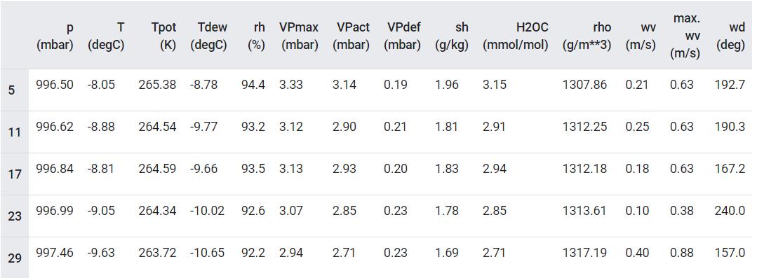
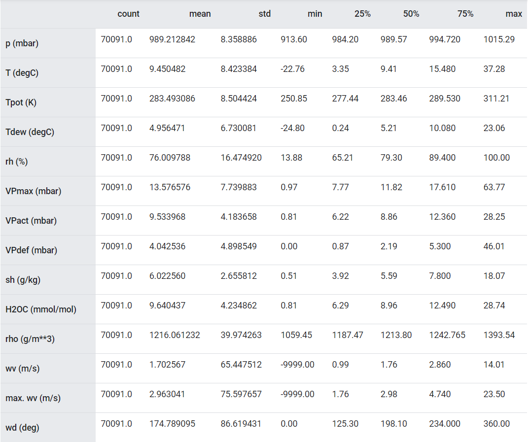
We will use a weather dataset containing 14 features such as air temperature, atmospheric pressure, and humidity to make predictions hourly. These were collected every 10 minutes, beginning in 2003.
One thing that should stand out is the min value of the wind velocity (wv (m/s)) and the maximum value (max. wv (m/s)) columns. This -9999 is likely erroneous.
There’s a separate wind direction column, so the velocity should be greater than zero (>=0). Replace it with zeros:
# The above inplace edits are reflected in the DataFrame. df['wv (m/s)'].min()
Feature engineering
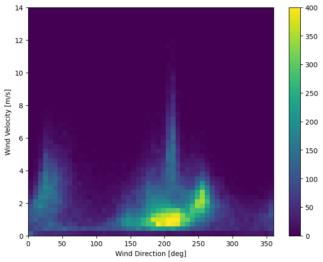
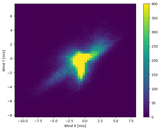
The last column of the data, wd (deg)—gives the wind direction in units of degrees. Angles do not make good model inputs: 360° and 0° should be close to each other and wrap around smoothly. Direction shouldn’t matter if the wind is not blowing.
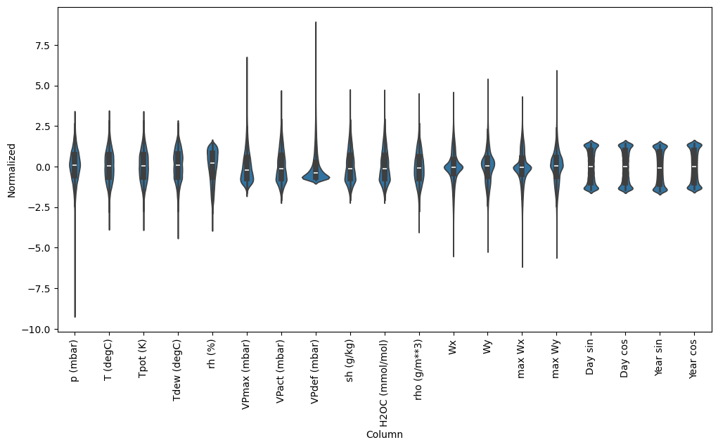
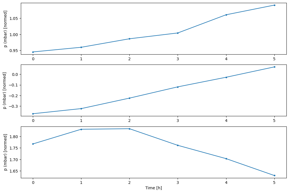
Right now the distribution of wind data looks like this:
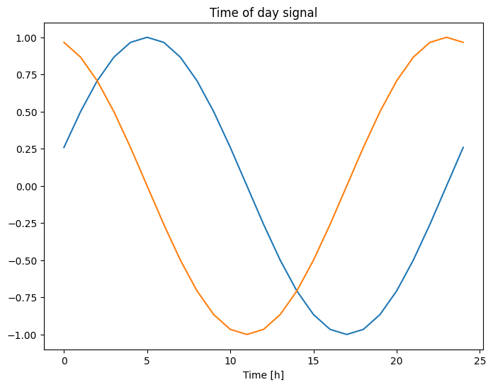
the time in seconds is not a useful model input. Being weather data, it has clear daily and yearly periodicity. And getting usable signals by using sine and cosine transforms to clear “Time of day” and “Time of year” signals:
We will be using a (70%, 20%, 10%) split for the training, validation, and test sets. And the data is not being randomly shuffled before splitting. This is for two reasons I think:
It ensures that chopping the data into windows of consecutive samples is still possible.
It ensures that the validation/test results are more realistic, being evaluated on the data collected after the model was trained.
1
2
3
4
5
6
7
8
column_indices = {name: i for i, name in enumerate(df.columns)}
class WindowGenerator(): def __init__(self, input_width, label_width, shift, train_df=train_df, val_df=val_df, test_df=test_df, label_columns=None): # Store the raw data. self.train_df = train_df self.val_df = val_df self.test_df = test_df
# Work out the label column indices. self.label_columns = label_columns if label_columns is not None: self.label_columns_indices = {name: i for i, name in enumerate(label_columns)} self.column_indices = {name: i for i, name in enumerate(train_df.columns)}
# Work out the window parameters. self.input_width = input_width self.label_width = label_width self.shift = shift
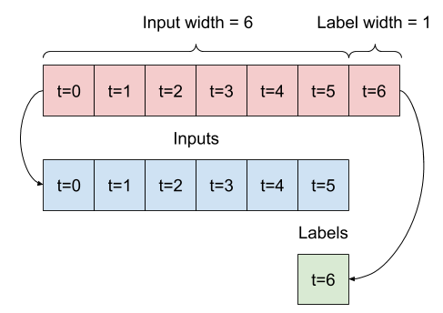
Given a list of consecutive inputs, the split_window method will convert them to a window of inputs and a window of labels.
The example w2 you define earlier will be split like this:
1 2 3 4 5 6 7 8 9 10 11 12 13 14 15 16 17
def split_window(self, features): inputs = features[:, self.input_slice, :] labels = features[:, self.labels_slice, :] if self.label_columns is not None: labels = tf.stack( [labels[:, :, self.column_indices[name]] for name in self.label_columns], axis=-1)
# Slicing doesn't preserve static shape information, so set the shapes # manually. This way the `tf.data.Datasets` are easier to inspect. inputs.set_shape([None, self.input_width, None]) labels.set_shape([None, self.label_width, None])
return inputs, labels
WindowGenerator.split_window = split_window
Test it out:
1 2 3 4 5 6 7 8 9 10 11
# Stack three slices, the length of the total window. example_window = tf.stack([np.array(train_df[:w2.total_window_size]), np.array(train_df[100:100+w2.total_window_size]), np.array(train_df[200:200+w2.total_window_size])])
The code above took a batch of three 7-time step windows with 19 features at each time step. It splits them into a batch of 6-time step 19-feature inputs, and a 1-time step 1-feature label. The label only has one feature because the WindowGenerator was initialized with label_columns=['T (degC)'].
Plot
Here is a plot method that allows a simple visualization of the split window:
@property def example(self): """Get and cache an example batch of `inputs, labels` for plotting.""" result = getattr(self, '_example', None) if result is None: # No example batch was found, so get one from the `.train` dataset result = next(iter(self.train)) # And cache it for next time self._example = result return result
WindowGenerator.train = train WindowGenerator.val = val WindowGenerator.test = test WindowGenerator.example = example
Now, the WindowGenerator object gives you access to the tf.data.Dataset objects, so we can easily iterate over the data.
1 2
# Each element is an (inputs, label) pair. w2.train.element_spec
for example_inputs, example_labels in w2.train.take(1): print(f'Inputs shape (batch, time, features): {example_inputs.shape}') print(f'Labels shape (batch, time, features): {example_labels.shape}')
1 2
Inputs shape (batch, time, features): (32, 6, 19) Labels shape (batch, time, features): (32, 1, 1)
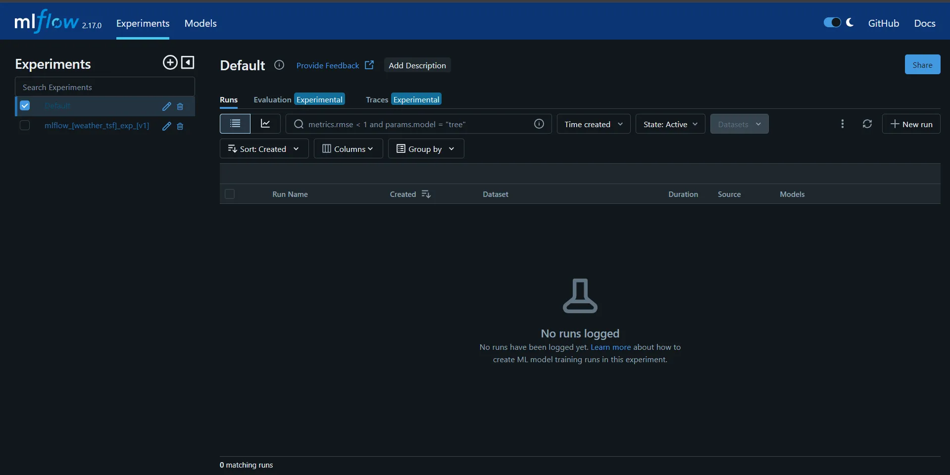
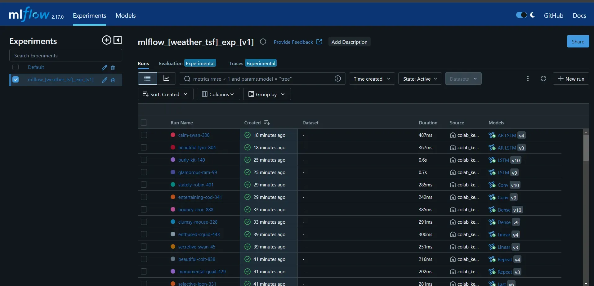
MLFLOW
before diving into next section, we will set up MLflow(open source MLOps platform) for tracking and logging the parameters and metrics for the models to be implemented and find out the potential model with best performance lining with the time series data
Install mlflow and pyngrok
1
!pip install mlflow pyngrok --quiet
Config pyngrok port and set up mlflow UI
1 2 3 4 5 6 7 8 9 10 11 12 13 14 15
from pyngrok import ngrok from getpass import getpass import mlflow # Terminate open tunnels if exist ngrok.kill()
#sign up a new pyngrok account for the AUTH token if not have NGROK_AUTH_TOKEN = getpass('Your_AUTH_TOKEN:') ngrok.set_auth_token(NGROK_AUTH_TOKEN)
# Open an HTTPs tunnel on port 5000 for http://localhost:5000 ngrok_tunnel = ngrok.connect(addr="5000", proto="http", bind_tls=True) print("MLflow Tracking UI:", ngrok_tunnel.public_url) get_ipython().system_raw("mlflow ui --port 5000 &") mlflow.set_experiment("mlflow_[weather_tsf]_exp_[v1]")
plt.title(f'Metrics with Val_df and Test_df for {model_type} Models') plt.xlabel('Metrics') plt.ylabel('Values') plt.legend(title=model_type) plt.tight_layout() plt.show()
Single step models
This blog will introduce two sorts of models, one for single step models with predicting one hour and the other for multi step models with predicting one day.
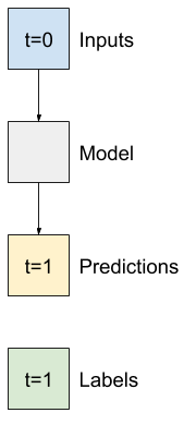
single step models predicts a single feature’s value—1 time step (one hour) into the future based only on the current conditions.
So, start by building models to predict the T (degC) value one hour into the future
Configure a WindowGenerator object to produce these single-step (input, label) pairs:
That printed some performance metrics, but those don’t give you a feeling for how well the model is doing.
The WindowGenerator has a plot method, but the plots won’t be very interesting with only a single sample.
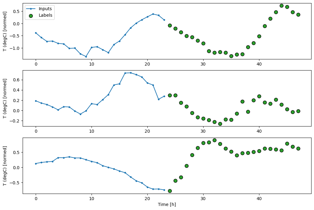
So, create a wider WindowGenerator that generates windows 24 hours of consecutive inputs and labels at a time. The new wide_window variable doesn’t change the way the model operates. The model still makes predictions one hour into the future based on a single input time step. Here, the time axis acts like the batch axis: each prediction is made independently with no interaction between time steps:
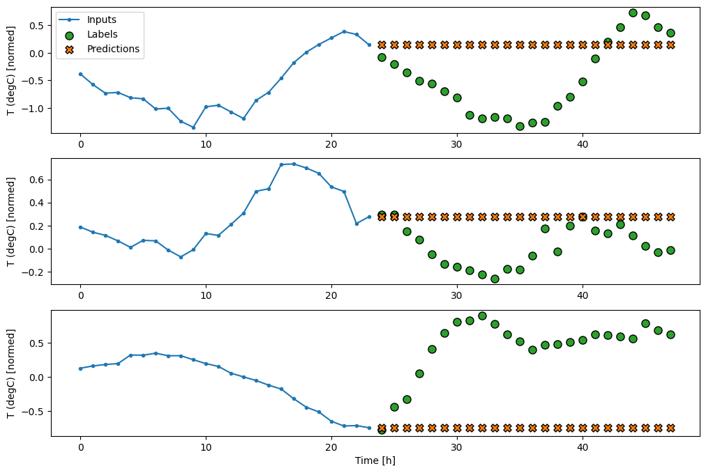
This expanded window can be passed directly to the same baseline model without any code changes. This is possible because the inputs and labels have the same number of time steps, and the baseline just forwards the input to the output:
1
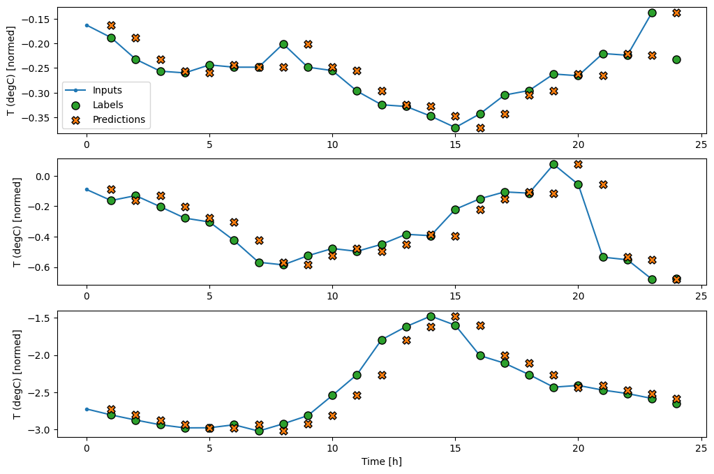
wide_window.plot(baseline)
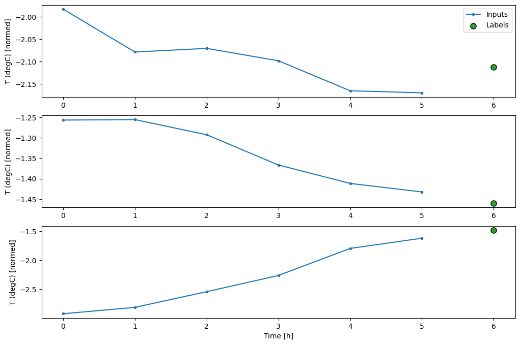
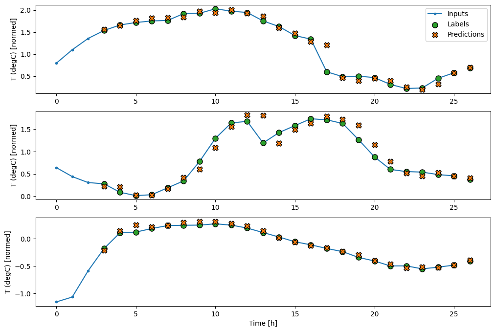
In the above plots of three examples the single step model is run over the course of 24 hours. This deserves some explanation:
The blue Inputs line shows the input temperature at each time step. The model receives all features, this plot only shows the temperature.
The green Labels dots show the target prediction value. These dots are shown at the prediction time, not the input time. That is why the range of labels is shifted 1 step relative to the inputs.
The orange Predictions crosses are the model’s prediction’s for each output time step. If the model were predicting perfectly the predictions would land directly on the Labels.
Linear model
A tf.keras.layers.Dense layer with no activation set is a linear model. The layer only transforms the last axis of the data from (batch, time, inputs) to (batch, time, units); it is applied independently to every item across the batch and time axes.
1 2 3
linear = tf.keras.Sequential([ tf.keras.layers.Dense(units=1) ])
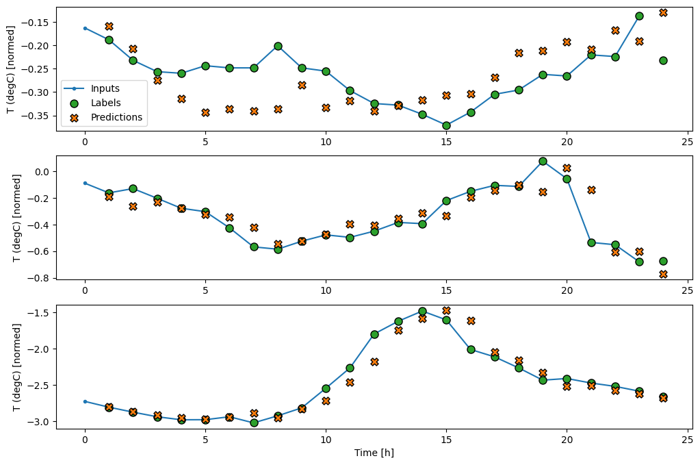
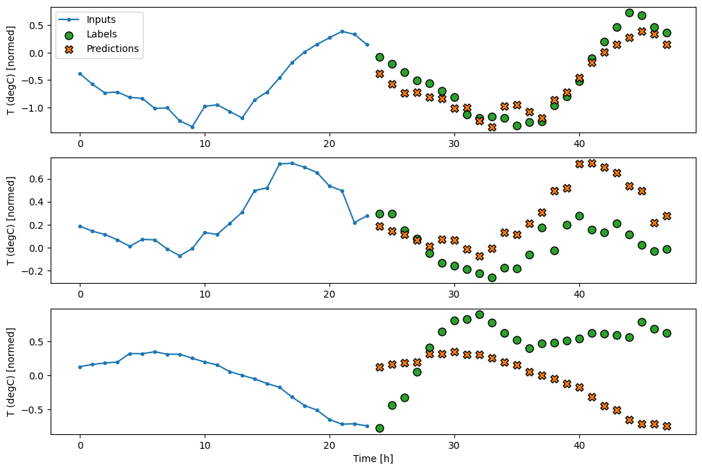
Here is the plot of its example predictions on the wide_window, and how in many cases the prediction is clearly better than just returning the input temperature, but in a few cases it’s worse:
1
wide_window.plot(linear)
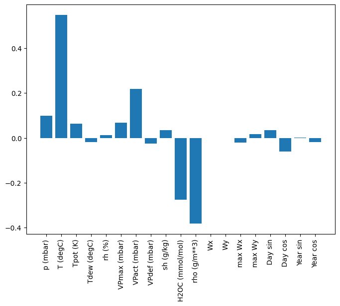
One advantage to linear models is that they’re relatively simple to interpret. We can pull out the layer’s weights and visualise the weight assigned to each input:
Sometimes the model doesn’t even place the most weight on the input T (degC). This is one of the risks of random initialisation.
Dense
Here’s a model similar to the linear model for checking the performance of deeper, more powerful, single input step models, except it stacks several a few Dense layers between the input and the output:
A single-time-step model has no context for the current values of its inputs. It can’t see how the input features are changing over time. To address this issue the model needs access to multiple time steps when making predictions:
The baseline, linear and dense models handled each time step independently. Here the model will take multiple time steps as input to produce a single output.
Create a WindowGenerator that will produce batches of three-hour inputs and one-hour labels:
training a dense model on a multiple-input-step window by adding a tf.keras.layers.Flatten as the first layer of the model:
1
2
3
4
5
6
7
8
9
10
multi_step_dense = tf.keras.Sequential([ # Shape: (time, features) => (time*features) tf.keras.layers.Flatten(), tf.keras.layers.Dense(units=32, activation='relu'), tf.keras.layers.Dense(units=32, activation='relu'), tf.keras.layers.Dense(units=1), # Add back the time dimension. # Shape: (outputs) => (1, outputs) tf.keras.layers.Reshape([1, -1]), ])
1 2 3
history = compile_and_fit(multi_step_dense, conv_window)
print("Conv model on `conv_window`") print('Input shape:', conv_window.example[0].shape) print('Output shape:', conv_model(conv_window.example[0]).shape)
1 2 3
Conv model on `conv_window` Input shape: (32, 3, 19) Output shape: (32, 1, 1)
check out the input and output tensor shape of wide_window
We could find out that the output is shorter than the input. To make training or plotting work, we need the labels, and prediction to have the same length. So build a WindowGenerator to produce wide windows with a few extra input time steps so the label and prediction lengths match:
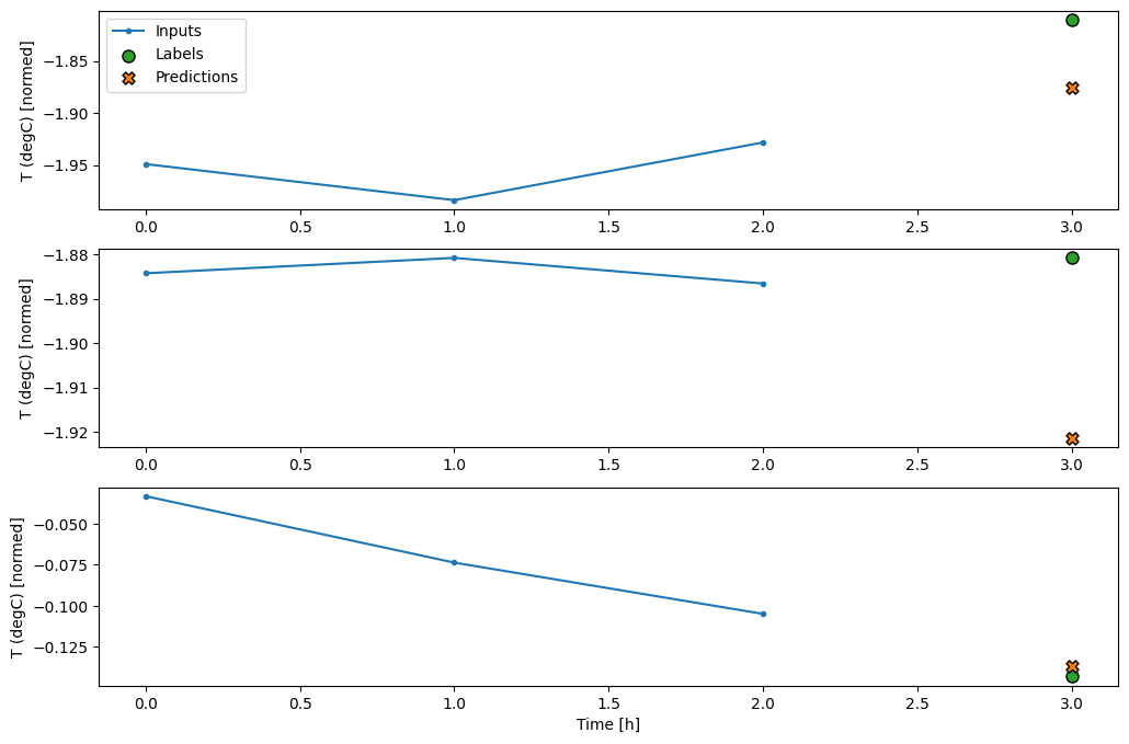
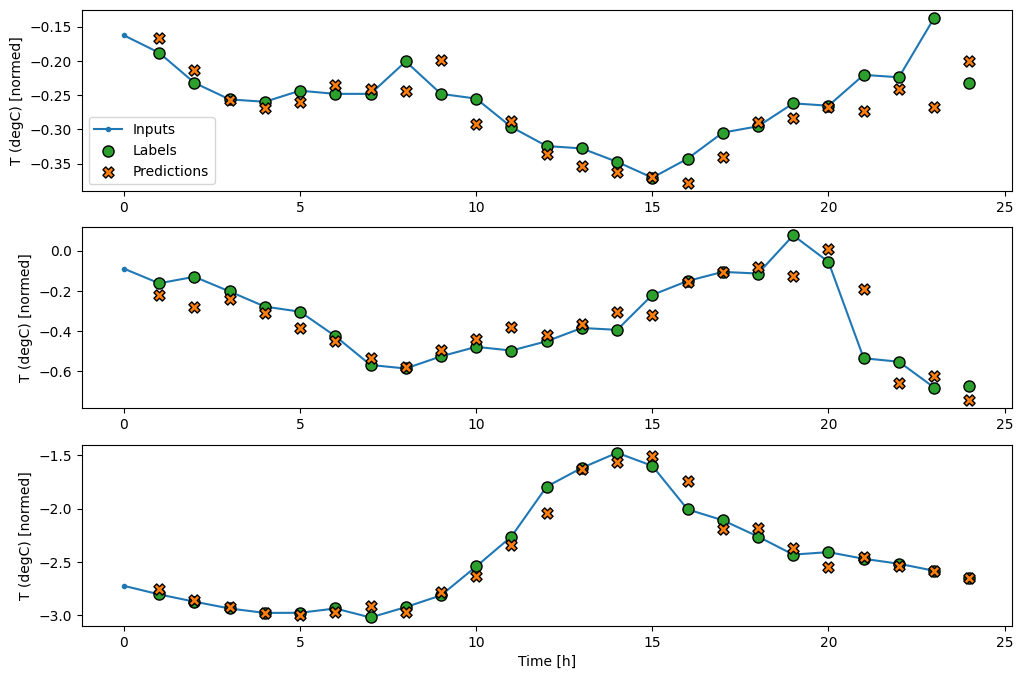
Every prediction here is based on the 3 preceding time steps:
1
wide_conv_window.plot(conv_model)
Recurrent neural network
A Recurrent Neural Network (RNN) is a type of neural network well-suited to time series data. RNNs process a time series step-by-step, maintaining an internal state from time-step to time-step. And we will use an RNN layer called Long Short-Term Memory (tf.keras.layers.LSTM).
n important constructor argument for all Keras RNN layers, such as tf.keras.layers.LSTM, is the return_sequences argument. This setting can configure the layer in one of two ways:
If False, the default, the layer only returns the output of the final time step, giving the model time to warm up its internal state before making a single prediction:
If True, the layer returns an output for each input. This is useful for:
Stacking RNN layers.
Training a model on multiple time steps simultaneously.
1 2 3 4 5 6
lstm_model = tf.keras.models.Sequential([ # Shape [batch, time, features] => [batch, time, lstm_units] tf.keras.layers.LSTM(32, return_sequences=True), # Shape => [batch, time, features] tf.keras.layers.Dense(units=1) ])
1 2 3 4 5
history = compile_and_fit(lstm_model, wide_window)
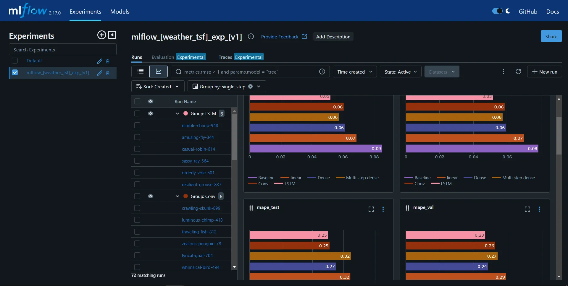
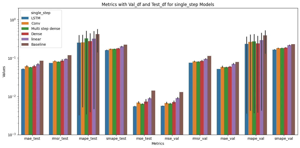
use MLFLOW plot func to present and analyse the metrics
1
plot_mlflow_metrics('single_step')
from the picture and we could find out the LSTM model metrics are better than other models’ based on the test and validation dataset according to the four different common used metrics in time series data prediction, which are mean_absolute_error, mean_square_error, mean_absolute_percentage_error, symmetric_mean_absolute_percentage_error and root_mean_square_error
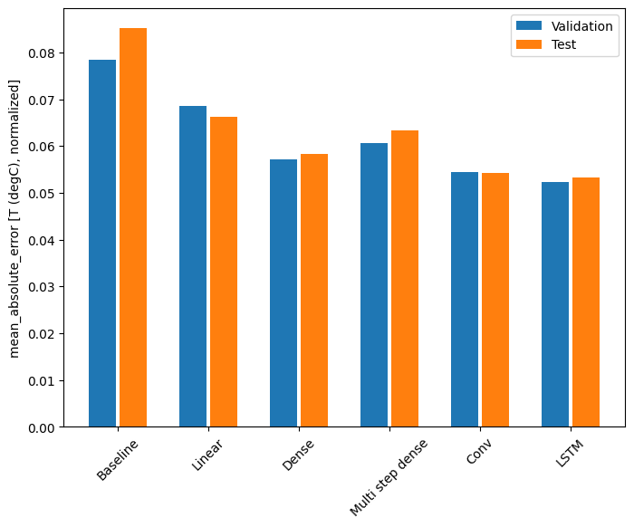
Diving into deeper on comparison of the mae metric for the models
x = np.arange(len(performance)) width = 0.3 metric_name = 'mean_absolute_error' val_mae = [v[metric_name] for v in val_performance.values()] test_mae = [v[metric_name] for v in performance.values()]
for name, value in performance.items(): print(f'{name:12s}: {value[metric_name]:0.4f}')
1 2 3 4 5 6
Baseline : 0.0852 Linear : 0.0663 Dense : 0.0584 Multi step dense: 0.0633 Conv : 0.0543 LSTM : 0.0533
With this dataset typically each of the models does slightly better than the one before it and
from the data, the performance of the model based on LSTM model is better than other’s, which is 0.0533, when predicting single time step.
Multi-step models
This section looks at how to expand these models to make multiple time step predictions.
In a multi-step prediction, the model needs to learn to predict a range of future values. Thus, unlike a single step model, where only a single future point is predicted, a multi-step model predicts a sequence of the future values.
There are two rough approaches to this:
Single shot predictions where the entire time series is predicted at once.
Autoregressive predictions where the model only makes single step predictions and its output is fed back as its input.
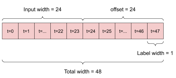
For the multi-step model, the training data again consists of hourly samples. However, here, the models will learn to predict 24 hours into the future, given 24 hours of the past.
Here is a Window object that generates these slices from the dataset:
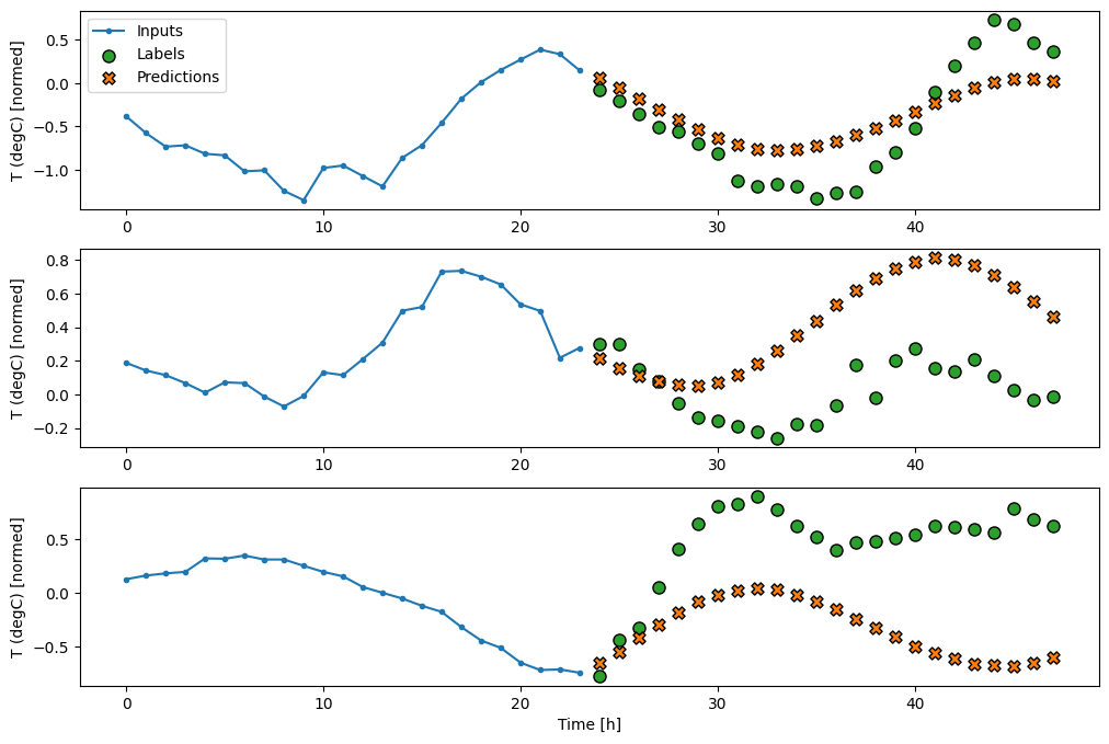
Since this task is to predict 24 hours into the future, given 24 hours of the past, another simple approach is to repeat the previous day, assuming tomorrow will be similar:
1 2 3 4 5 6 7 8 9 10 11
class RepeatBaseline(tf.keras.Model): def call(self, inputs): return inputs
A simple linear model based on the last input time step does better than either baseline, but is underpowered. The model needs to predict OUTPUT_STEPS time steps, from a single input time step with a linear projection. It can only capture a low-dimensional slice of the behavior, likely based mainly on the time of day and time of year.
1 2 3 4 5 6 7 8 9 10 11 12 13 14 15 16 17 18
multi_linear_model = tf.keras.Sequential([ # Take the last time-step. # Shape [batch, time, features] => [batch, 1, features] tf.keras.layers.Lambda(lambda x: x[:, -1:, :]), # Shape => [batch, 1, out_steps*features] tf.keras.layers.Dense(OUT_STEPS*num_features, kernel_initializer=tf.initializers.zeros()), # Shape => [batch, out_steps, features] tf.keras.layers.Reshape([OUT_STEPS, num_features]) ])
history = compile_and_fit(multi_linear_model, multi_window)
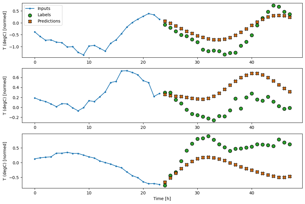
A convolutional model makes predictions based on a fixed-width history, which may lead to better performance than the dense model since it can see how things are changing over time:
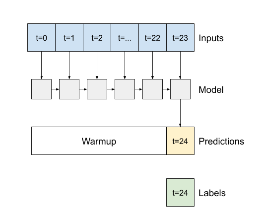
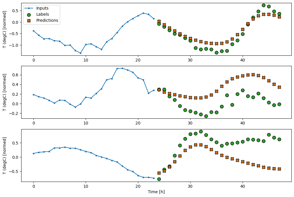
A recurrent model can learn to use a long history of inputs, if it’s relevant to the predictions the model is making. Here the model will accumulate internal state for 24 hours, before making a single prediction for the next 24 hours. In this single-shot format, the LSTM only needs to produce an output at the last time step, so set return_sequences=False in tf.keras.layers.LSTM.
In this multi-step format, the LSTM only needs to produce an output at the last time step, so set return_sequences=False in tf.keras.layers.LSTM.
1 2 3 4 5 6 7 8 9 10 11 12 13 14 15 16 17 18
multi_lstm_model = tf.keras.Sequential([ # Shape [batch, time, features] => [batch, lstm_units]. # Adding more `lstm_units` just overfits more quickly. tf.keras.layers.LSTM(32, return_sequences=False), # Shape => [batch, out_steps*features]. tf.keras.layers.Dense(OUT_STEPS*num_features, kernel_initializer=tf.initializers.zeros()), # Shape => [batch, out_steps, features]. tf.keras.layers.Reshape([OUT_STEPS, num_features]) ])
history = compile_and_fit(multi_lstm_model, multi_window)
The above models all predict the entire output sequence in a single step.
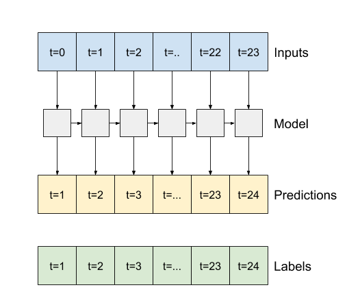
In some cases it may be helpful for the model to decompose this prediction into individual time steps. Then, each model’s output can be fed back into itself at each step and predictions can be made conditioned on the previous one.
The model will have the same basic form as the single-step LSTM models from earlier: a tf.keras.layers.LSTM layer followed by a tf.keras.layers.Dense layer that converts the LSTM layer’s outputs to model predictions.
In this case, the model has to manually manage the inputs for each step, so it uses tf.keras.layers.LSTMCell directly for the lower level, single time step interface.
1 2 3 4 5 6 7 8 9 10
class FeedBack(tf.keras.Model): def __init__(self, units, out_steps): super().__init__() self.out_steps = out_steps self.units = units self.lstm_cell = tf.keras.layers.LSTMCell(units) # Also wrap the LSTMCell in an RNN to simplify the `warmup` method. self.lstm_rnn = tf.keras.layers.RNN(self.lstm_cell, return_state=True) self.dense = tf.keras.layers.Dense(num_features) feedback_model = FeedBack(units=32, out_steps=OUT_STEPS)
The first method this model needs is a warmup method to initialize its internal state based on the inputs. Once trained, this state will capture the relevant parts of the input history. This is equivalent to the single-step LSTM model from earlier
def call(self, inputs, training=None): # Use a TensorArray to capture dynamically unrolled outputs. predictions = [] # Initialize the LSTM state. prediction, state = self.warmup(inputs)
# Insert the first prediction. predictions.append(prediction)
# Run the rest of the prediction steps. for n in range(1, self.out_steps): # Use the last prediction as input. x = prediction # Execute one lstm step. x, state = self.lstm_cell(x, states=state, training=training) # Convert the lstm output to a prediction. prediction = self.dense(x) # Add the prediction to the output. predictions.append(prediction)
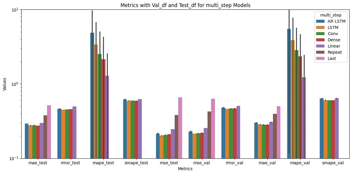
LSTM model performs well generally except on mean_abosolute_percentage_error.
1 2 3 4 5 6 7 8 9 10 11 12 13 14
x = np.arange(len(multi_performance)) width = 0.3
metric_name = 'mean_absolute_error' val_mae = [v[metric_name] for v in multi_val_performance.values()] test_mae = [v[metric_name] for v in multi_performance.values()]
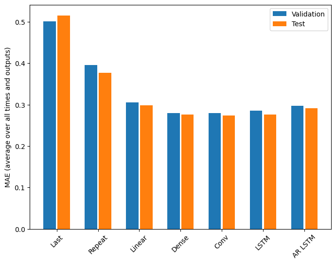
plt.bar(x - 0.17, val_mae, width, label='Validation') plt.bar(x + 0.17, test_mae, width, label='Test') plt.xticks(ticks=x, labels=multi_performance.keys(), rotation=45) plt.ylabel(f'MAE (average over all times and outputs)') _ = plt.legend()
1 2
for name, value in multi_performance.items(): print(f'{name:8s}: {value[metric_name]:0.4f}')
1 2 3 4 5 6 7
Last    : 0.5157
Repeat  : 0.3774
Linear  : 0.2980
Dense   : 0.2765
Conv    : 0.2732
LSTM    : 0.2767
AR LSTM : 0.2910
The gains achieved going from a dense model to convolutional and recurrent models are only a few percent (if any), and the autoregressive model performed clearly worse. So these more complex approaches may not be worth while on this problem, but there was no way to know without trying.
Finally, we will use LSTM model to implement our time series data forecasting. Checking out the GitHub repo below for complete implementing LSTM model with the configs above on the prediction tasks and the blog: Deploy the model on Kubeflow
• Environment and dependencies set up • Exploratory Data Analysis • Configure MLflow for model evaluation and model metrics visualisation • Compile, fit, train and evaluate the models with single step type • Compile, fit, train and evaluate the models with multi step type • Compare the metrics for choosing best performance model among them