Neural style transfer

Introduction

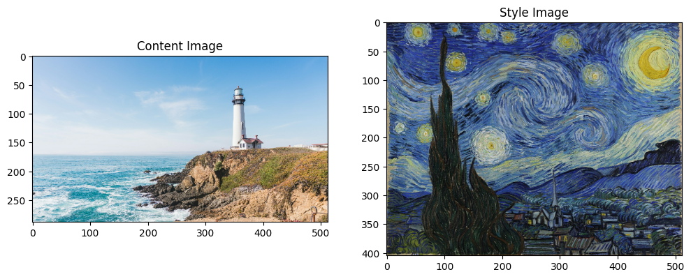
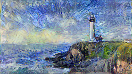
Neural style transfer is an optimisation technique used to take two images—a content image and a style reference image (such as an artwork by a famous painter)—and blend them together so the output image looks like the content image, but “painted” in the style of the style reference image.

This is implemented by using tensorflow pretrained model VGG19, accessing and changing the intermediate layers of the model, extracting style and content, running gradient descent to minimise the loss function: total variation loss with explicit regularisation to reduce high-frequency artifacts and preserve edge details, and optimising the output image to match the statistics of the content and the style reference image. These statistics are extracted from the images using a convolutional network.

Configuration

jupyter notebook
Python 3.10.12
matplotlib==3.7.1
Pillow==10.4.0
numpy==1.26.4
requests==2.32.3
tensorflow==2.17.0

Setup

import os
import tensorflow as tf

import IPython.display as display

import matplotlib.pyplot as plt
import matplotlib as mpl
mpl.rcParams['figure.figsize'] = (12, 12)
mpl.rcParams['axes.grid'] = False

import numpy as np
import PIL.Image
import time
import functools

#tensor_to_image
def tensor_to_image(tensor):
  #convert pixel values from the range [0,1] to [0,255]
  tensor = tensor*255
  tensor = np.array(tensor, dtype=np.uint8)
  if np.ndim(tensor)>3:
    assert tensor.shape[0] == 1
    tensor = tensor[0]
  return PIL.Image.fromarray(tensor)

Download content and style image

content_path = tf.keras.utils.get_file('lighthouse.jpg', 'https://unsplash.com/photos/l5b_Jd8Ttfg/download?ixid=M3wxMjA3fDB8MXxhbGx8fHx8fHx8fHwxNzI5NTI3OTk1fA&force=true&w=2400')
style_path = tf.keras.utils.get_file('starrynight.png','https://upload.wikimedia.org/wikipedia/commons/thumb/e/ea/Van_Gogh_-_Starry_Night_-_Google_Art_Project.jpg/1024px-Van_Gogh_-_Starry_Night_-_Google_Art_Project.jpg')

Visualise the input

Define a function to load an image and limit its maximum dimension to 512 pixels.

def load_img(path_to_img):
  max_dim = 512
  img = tf.io.read_file(path_to_img)
  img = tf.image.decode_image(img, channels=3)
  img = tf.image.convert_image_dtype(img, tf.float32)

  shape = tf.cast(tf.shape(img)[:-1], tf.float32)
  long_dim = max(shape)
  scale = max_dim / long_dim

  new_shape = tf.cast(shape * scale, tf.int32)

  img = tf.image.resize(img, new_shape)
  img = img[tf.newaxis, :]
  return img

Create a simple function to display an image:

def imshow(image, title=None):
  if len(image.shape) > 3:
    image = tf.squeeze(image, axis=0)

  plt.imshow(image)
  if title:
    plt.title(title)

content_image = load_img(content_path)
style_image = load_img(style_path)

plt.subplot(1, 2, 1)
imshow(content_image, 'Content Image')

plt.subplot(1, 2, 2)
imshow(style_image, 'Style Image')

Define content and style representations

We will be using the VGG19 network architecture, a pretrained image classification network to implement it and use the intermediate layers of the model to get the content and style representations of the image. Starting from the network’s input layer, the first few layer activations represent low-level features like edges and textures. With stepping through the network, the final few layers represent higher-level features.

Load a VGG19 and test run it on our image to ensure it’s used correctly:

x = tf.keras.applications.vgg19.preprocess_input(content_image*255)
x = tf.image.resize(x, (224, 224))
vgg = tf.keras.applications.VGG19(include_top=True, weights='imagenet')
prediction_probabilities = vgg(x)
prediction_probabilities.shape

#TensorShape([1, 1000])

predicted_top_5 = tf.keras.applications.vgg19.decode_predictions(prediction_probabilities.numpy())[0]
[(class_name, prob) for (number, class_name, prob) in predicted_top_5]

#class_name, prob
"""
[('beacon', 0.5217742),
 ('promontory', 0.3035163),
 ('cliff', 0.09787675),
 ('breakwater', 0.04300915),
 ('seashore', 0.014805787)]
""" 

 load a VGG19 without the classification head, and list the layer names

vgg = tf.keras.applications.VGG19(include_top=False, weights='imagenet')

print()
for layer in vgg.layers:
  print(layer.name)
#layer.name
"""
input_layer_1
block1_conv1
block1_conv2
block1_pool
block2_conv1
block2_conv2
block2_pool
block3_conv1
block3_conv2
block3_conv3
block3_conv4
block3_pool
block4_conv1
block4_conv2
block4_conv3
block4_conv4
block4_pool
block5_conv1
block5_conv2
block5_conv3
block5_conv4
block5_pool
"""

Choose intermediate layers from the network to represent the style and content of the image:

content_layers = ['block5_conv2'] 

style_layers = ['block1_conv1',
                'block2_conv1',
                'block3_conv1', 
                'block4_conv1', 
                'block5_conv1']

num_content_layers = len(content_layers)
num_style_layers = len(style_layers)

Intermediate layers for style and content

So why do these intermediate outputs within our pretrained image classification network allow us to define style and content representations?

Here is a paragraph for the explains reference from Tensorflow Docs:

At a high level, in order for a network to perform image classification (which this network has been trained to do), it must understand the image. This requires taking the raw image as input pixels and building an internal representation that converts the raw image pixels into a complex understanding of the features present within the image.

This is also a reason why convolutional neural networks are able to generalize well: they’re able to capture the invariances and defining features within classes (e.g. cats vs. dogs) that are agnostic to background artifacts and other nuisances. Thus, somewhere between where the raw image is fed into the model and the output classification label, the model serves as a complex feature extractor. By accessing intermediate layers of the model, we’re able to describe the content and style of input images.

Build the model

builds a VGG19 model that returns a list of intermediate layer outputs through specifying the inputs and outputs

def vgg_layers(layer_names):
  """ Creates a VGG model that returns a list of intermediate output values."""
  # Load our model. Load pretrained VGG, trained on ImageNet data
  vgg = tf.keras.applications.VGG19(include_top=False, weights='imagenet')
  vgg.trainable = False
  
  outputs = [vgg.get_layer(name).output for name in layer_names]

  model = tf.keras.Model([vgg.input], outputs)
  return model
  
#create the model
style_extractor = vgg_layers(style_layers)
style_outputs = style_extractor(style_image*255)

#Look at the statistics of each layer's output
for name, output in zip(style_layers, style_outputs):
  print(name)
  print("  shape: ", output.numpy().shape)
  print("  min: ", output.numpy().min())
  print("  max: ", output.numpy().max())
  print("  mean: ", output.numpy().mean())
  print()

#each layer's outputs
"""
block1_conv1
  shape:  (1, 405, 512, 64)
  min:  0.0
  max:  660.528
  mean:  23.849983

block2_conv1
  shape:  (1, 202, 256, 128)
  min:  0.0
  max:  2981.8281
  mean:  147.914

block3_conv1
  shape:  (1, 101, 128, 256)
  min:  0.0
  max:  7421.774
  mean:  144.3642

block4_conv1
  shape:  (1, 50, 64, 512)
  min:  0.0
  max:  16733.793
  mean:  560.6592

block5_conv1
  shape:  (1, 25, 32, 512)
  min:  0.0
  max:  3804.7947
  mean:  48.127247
"""

Calculate style

The content of an image is represented by the values of the intermediate feature maps.

It turns out, the style of an image can be described by the means and correlations across the different feature maps. Calculate a Gram matrix that includes this information by taking the outer product of the feature vector with itself at each location, and averaging that outer product over all locations. This Gram matrix can be calculated for a particular layer as:

• represents the Gram matrix element for feature map and feature map at layer . It quantifies the correlation between feature maps and
• and are the activation values of feature map and feature map at position. By calculating their outer product, We can capture the joint information of these two feature maps at that position.
• By summing the outer products over all positions and the dividing by (the spatial dimensions of the feature maps), and then we can obtain the average correlation between the feature maps.

And it could be implemented by using the tf.linalg.einsum function

def gram_matrix(input_tensor):
  result = tf.linalg.einsum('bijc,bijd->bcd', input_tensor, input_tensor)
  input_shape = tf.shape(input_tensor)
  num_locations = tf.cast(input_shape[1]*input_shape[2], tf.float32)
  return result/(num_locations)

Extract style and content

Build a model that returns the style and content tensors.

class StyleContentModel(tf.keras.models.Model):
  def __init__(self, style_layers, content_layers):
    super(StyleContentModel, self).__init__()
    self.vgg = vgg_layers(style_layers + content_layers)
    self.style_layers = style_layers
    self.content_layers = content_layers
    self.num_style_layers = len(style_layers)
    self.vgg.trainable = False

  def call(self, inputs):
    "Expects float input in [0,1]"
    inputs = inputs*255.0
    preprocessed_input = tf.keras.applications.vgg19.preprocess_input(inputs)
    outputs = self.vgg(preprocessed_input)
    style_outputs, content_outputs = (outputs[:self.num_style_layers],
                                      outputs[self.num_style_layers:])

    style_outputs = [gram_matrix(style_output)
                     for style_output in style_outputs]

    content_dict = {content_name: value
                    for content_name, value
                    in zip(self.content_layers, content_outputs)}

    style_dict = {style_name: value
                  for style_name, value
                  in zip(self.style_layers, style_outputs)}

    return {'content': content_dict, 'style': style_dict}

When called on an image, this model returns the gram matrix (style) of the style_layers and content of the content_layers:

extractor = StyleContentModel(style_layers, content_layers)

results = extractor(tf.constant(content_image))

print('Styles:')
for name, output in sorted(results['style'].items()):
  print("  ", name)
  print("    shape: ", output.numpy().shape)
  print("    min: ", output.numpy().min())
  print("    max: ", output.numpy().max())
  print("    mean: ", output.numpy().mean())
  print()

print("Contents:")
for name, output in sorted(results['content'].items()):
  print("  ", name)
  print("    shape: ", output.numpy().shape)
  print("    min: ", output.numpy().min())
  print("    max: ", output.numpy().max())
  print("    mean: ", output.numpy().mean())
  
#outputs
"""
Styles:
   block1_conv1
    shape:  (1, 64, 64)
    min:  0.15344943
    max:  63351.805
    mean:  709.7667

   block2_conv1
    shape:  (1, 128, 128)
    min:  0.0
    max:  143030.39
    mean:  17212.434

   block3_conv1
    shape:  (1, 256, 256)
    min:  0.0
    max:  535053.25
    mean:  13304.491

   block4_conv1
    shape:  (1, 512, 512)
    min:  0.0
    max:  4746262.0
    mean:  204897.52

   block5_conv1
    shape:  (1, 512, 512)
    min:  0.0
    max:  155404.47
    mean:  1599.2406

Contents:
   block5_conv2
    shape:  (1, 18, 32, 512)
    min:  0.0
    max:  2180.7375
    mean:  13.492043
"""

Run gradient descent

Gradient descent is an optimisation algorithm used to minimise a loss function. During the training of deep learning models, gradient descent proceeds through the following steps:

• Calculate Loss: First, compute the loss based on the difference between the model’s output and the true labels.
• Compute Gradients: Then, use the backpropagation algorithm to calculate the gradients of the loss function with respect to the model parameters.
• Update Parameters: Finally, use these gradients to update the model parameters, thus reducing the loss.

In tasks using VGG19 (like feature extraction), we may leverage a pre-trained model and fine-tune it to optimize performance for a specific task.

Set the style and content target values:

style_targets = extractor(style_image)['style']
content_targets = extractor(content_image)['content']

#Define a tf.Variable to contain the image to optimize. 
image = tf.Variable(content_image)

#Since this is a float image, define a function to keep the pixel values between 0 and 1:
def clip_0_1(image):
  return tf.clip_by_value(image, clip_value_min=0.0, clip_value_max=1.0)
  
# create an optimizer, both LBFGS and Adam are acceptable
opt = tf.keras.optimizers.Adam(learning_rate=0.02, beta_1=0.99, epsilon=1e-1)

# To optimize this, we will use a weighted combination of the two losses to get the total loss:
style_weight=1e-2
content_weight=1e4
def style_content_loss(outputs):
    style_outputs = outputs['style']
    content_outputs = outputs['content']
    style_loss = tf.add_n([tf.reduce_mean((style_outputs[name]-style_targets[name])**2) 
                           for name in style_outputs.keys()])
    style_loss *= style_weight / num_style_layers

    content_loss = tf.add_n([tf.reduce_mean((content_outputs[name]-content_targets[name])**2) 
                             for name in content_outputs.keys()])
    content_loss *= content_weight / num_content_layers
    loss = style_loss + content_loss
    return loss
# And finally use tf.GradientTape to update the image.
@tf.function()
def train_step(image):
  with tf.GradientTape() as tape:
    outputs = extractor(image)
    loss = style_content_loss(outputs)

  grad = tape.gradient(loss, image)
  opt.apply_gradients([(grad, image)])
  image.assign(clip_0_1(image))

Now run a few steps to test:

train_step(image)
train_step(image)
train_step(image)
tensor_to_image(image)

performing a longer optimisation

import time
start = time.time()

epochs = 10
steps_per_epoch = 100

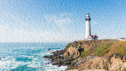
step = 0
for n in range(epochs):
  for m in range(steps_per_epoch):
    step += 1
    train_step(image)
    print(".", end='', flush=True)
  display.clear_output(wait=True)
  display.display(tensor_to_image(image))
  print("Train step: {}".format(step))
  
end = time.time()
print("Total time: {:.1f}".format(end-start))

Train step: 1000
Total time: 5952.3

Total variation loss

Variation loss is often used in image generation tasks, particularly in style transfer. Its primary aim is to maintain the smoothness and structure of the image while preventing excessive smoothing that could result in loss of detail. Variation loss is typically calculated based on the differences between pixel values, encouraging small changes between adjacent pixels. The formula can be expressed as:

Here, is the generated image, and and are the pixel coordinates of the image. This loss penalises large variations to maintain the natural smoothness of the image.

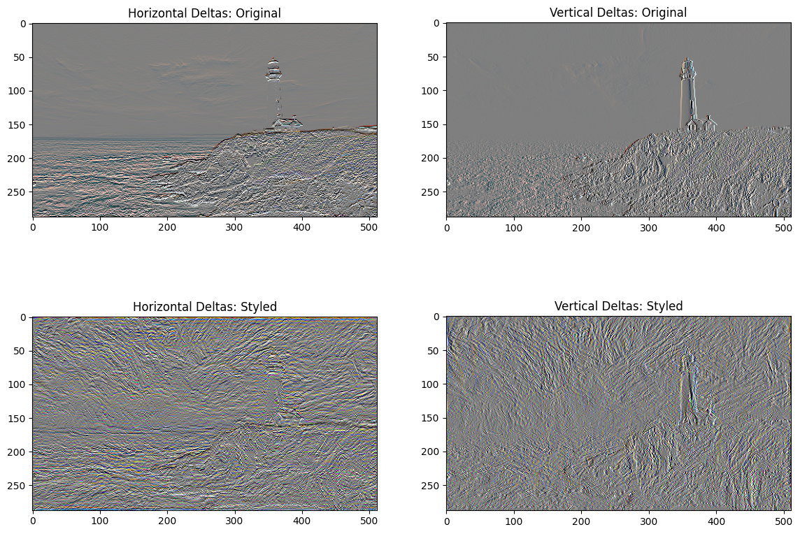
One downside to this basic implementation is that it produces a lot of high frequency artifacts. Decrease these using an explicit regularisation term on the high frequency components of the image.

def high_pass_x_y(image):
  x_var = image[:, :, 1:, :] - image[:, :, :-1, :]
  y_var = image[:, 1:, :, :] - image[:, :-1, :, :]

  return x_var, y_var

x_deltas, y_deltas = high_pass_x_y(content_image)

plt.figure(figsize=(14, 10))
plt.subplot(2, 2, 1)
imshow(clip_0_1(2*y_deltas+0.5), "Horizontal Deltas: Original")

plt.subplot(2, 2, 2)
imshow(clip_0_1(2*x_deltas+0.5), "Vertical Deltas: Original")

x_deltas, y_deltas = high_pass_x_y(image)

plt.subplot(2, 2, 3)
imshow(clip_0_1(2*y_deltas+0.5), "Horizontal Deltas: Styled")

plt.subplot(2, 2, 4)
imshow(clip_0_1(2*x_deltas+0.5), "Vertical Deltas: Styled")

This shows how the high frequency components have increased.

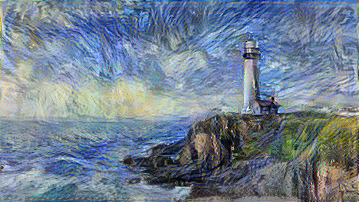
Re-run the optimisation

By minimizing the loss function incorporating total variation regularisation using gradient descent, we can effectively reduce high-frequency artifacts in images while preserving edge details.

# Choose a weight for the total_variation_loss
total_variation_weight=30

@tf.function()
def train_step(image):
  with tf.GradientTape() as tape:
    outputs = extractor(image)
    loss = style_content_loss(outputs)
    loss += total_variation_weight*tf.image.total_variation(image)

  grad = tape.gradient(loss, image)
  opt.apply_gradients([(grad, image)])
  image.assign(clip_0_1(image))
  
# Reinitialize the image-variable and the optimizer:
opt = tf.keras.optimizers.Adam(learning_rate=0.02, beta_1=0.99, epsilon=1e-1)
image = tf.Variable(content_image)

# Run the optimisation
import time
start = time.time()

epochs = 10
steps_per_epoch = 100

step = 0
for n in range(epochs):
  for m in range(steps_per_epoch):
    step += 1
    train_step(image)
    print(".", end='', flush=True)
  display.clear_output(wait=True)
  display.display(tensor_to_image(image))
  print("Train step: {}".format(step))

end = time.time()
print("Total time: {:.1f}".format(end-start))

Train step: 1000
Total time: 6952.3

Save the model

tf.saved_model.save(extractor, '/home/sagemaker-user/model/vgg19/model_file')

GitHub

Checking out the GitHub repo below for complete implementing VGG19 model with the configs above on the neural style transfer tasks and the blog: Deploy the model on AWS Sagemaker

https://github.com/PaddyZz/Neural-style-transfer

Conclusion

We have finished:

• Enviroment and dependencies set up
• Visualise the input images
• Define content and style image representations
• Configure the VGG19 intermediate layers
• Build the VGG19 model
• Calculate and extract style and content
• Run gradient descent
• Total variation loss
• Re-run the optimisation
• Save the model on AWS sagemaker jupyter notebook server directory

References

neural style transfer