ConvNets
Introduction
Convolutional Neural Networks (ConvNet/CNN) are a type of deep learning algorithm that can take input images, assign importance (learnable weights and biases) to various aspects/objects in the images, and distinguish between them. Compared to other classification algorithms, ConvNet requires much less preprocessing. While filters were originally designed manually, ConvNet has the ability to learn these filters/features through sufficient training.
The architecture of convolutional networks is inspired by the connection patterns of neurons in the human brain, particularly the organization of the visual cortex. A single neuron responds to stimuli only within a limited region of its visual field known as the receptive field. These fields overlap to cover the entire visual area.
Input Image
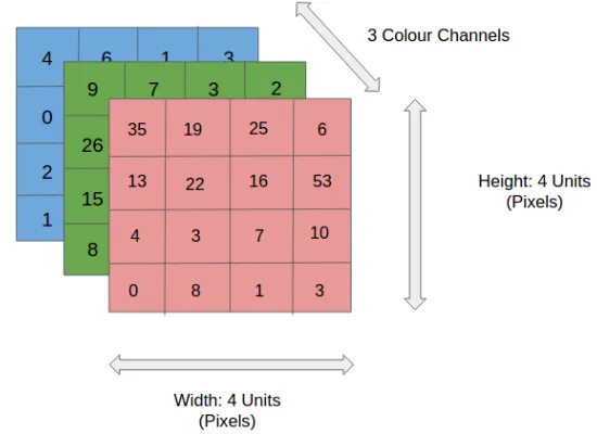
In the illustration, we have an RGB image that is divided into three color planes (red, green, and blue). There are many such color spaces for images—grayscale, RGB, HSV, CMYK, etc.
One can imagine the computational load when an image reaches 8K (7680×4320) resolution. The role of ConvNet is to simplify the image into a more manageable form without losing features critical for making accurate predictions. This is especially important when designing an architecture that not only excels at learning features but can also scale to vast datasets.
Convolutional Layer - The Kernel
Image Size = 5 (Height) x 5 (Width) x 1 (Number of Channels, e.g., RGB)
In the above illustration, the green portion resembles our 5x5x1 input image I. The elements involved in the convolution operation in the first part of the convolution layer are called the kernel/filter K, highlighted in yellow. We choose K as a 3x3x1 matrix.
With a stride length of 1 (non-strided), we perform element-wise multiplication between K and the image section P under the kernel Hadamard Product, moving the kernel 9 times.
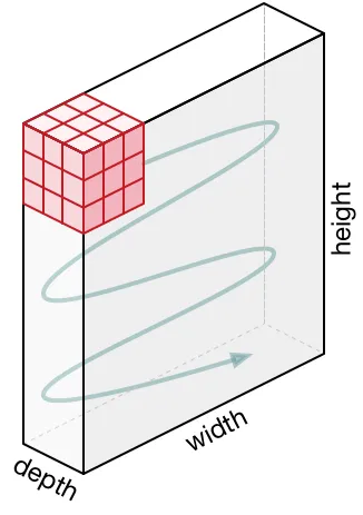
The filter moves to the right with a fixed stride value until it covers the entire width of the image. Then, it jumps back to the start (left side) of the image using the same stride value and repeats the process until the entire image is traversed.
For images with multiple channels (e.g., RGB), the kernel has the same depth as the input image. Matrix multiplication is performed between Kn and In stacks ([K1, I1]; [K2, I2]; [K3, I3]), summing all results with the bias to produce a compressed single-depth channel convolution feature output.
The purpose of the convolution operation is to extract high-level features from the input image, such as edges. Convolutional networks are not limited to just one convolution layer. Traditionally, the first ConvLayer captures low-level features like edges, colors, and gradient directions. By adding more layers, the architecture adapts to capture high-level features, providing us with a network that comprehensively understands images in the dataset, akin to human perception.
This operation can yield two types of results: one where the dimensions of the convolution features are reduced compared to the input, and another where dimensions are increased or remain unchanged. This is achieved by applying valid padding in the former case and same padding in the latter.
When we enhance a 5x5x1 image to a 6x6x1 image and then apply a 3x3x1 kernel on it, we find that the size of the convolution matrix is 5x5x1, hence the term Same Padding.
On the other hand, if we perform the same operation without any padding, we obtain a matrix with the dimensions of the kernel (3x3x1) itself, referred to as Valid Padding.
Pooling Layer
Similar to the convolutional layer, the pooling layer is responsible for reducing the spatial dimensions of the convolutional features. This is done to decrease the computational power needed for processing the data through dimensionality reduction. Additionally, it is useful for extracting dominant features that are invariant to rotation and position, thereby maintaining an effective training process for the model.
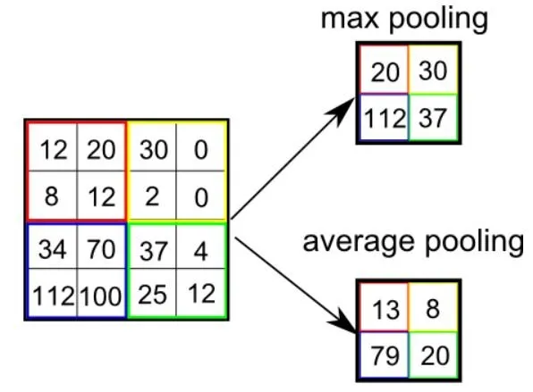
There are two types of pooling: max pooling and average pooling. Max pooling returns the maximum value from the portion of the image covered by the kernel. On the other hand, average pooling returns the average of all values in the portion of the image covered by the kernel.
Max pooling can also act as a noise suppressor. It completely discards noisy activations and performs denoising along with dimensionality reduction. In contrast, average pooling simply reduces dimensions as a noise suppression mechanism. Therefore, we can say that max pooling performs significantly better than average pooling.
The convolutional layer and pooling layer together form the i-th layer of the convolutional neural network. Depending on the complexity of the image, the number of such layers can be increased to further capture low-level details, but this comes at the cost of requiring more computational power.
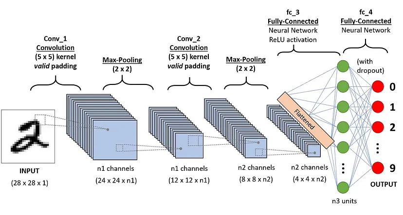
After the above processes, we have successfully enabled the model to understand features. Next, we will flatten the final output and input it into a standard neural network for classification.
Classification — Fully Connected Layer (FC Layer)
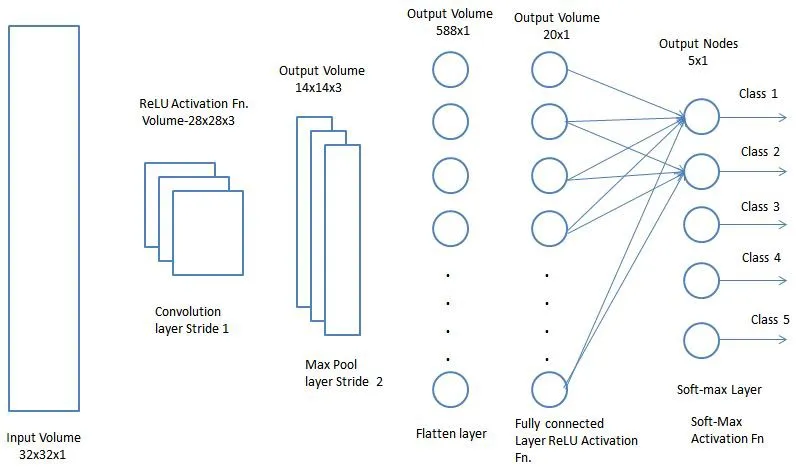
Adding a fully connected layer is a (typically) inexpensive way to learn a nonlinear combination of the high-level features represented by the output of the convolutional layers. The fully connected layer learns the possible nonlinear functions in that space.
Now that we have transformed the input image into a format suitable for a multilayer perceptron, we will flatten the image into a column vector. The flattened output is fed into a feedforward neural network, and backpropagation is applied in each iteration of training. Over a series of epochs, the model becomes capable of distinguishing between the main features in the image and certain low-level features, classifying them using Softmax classification techniques.